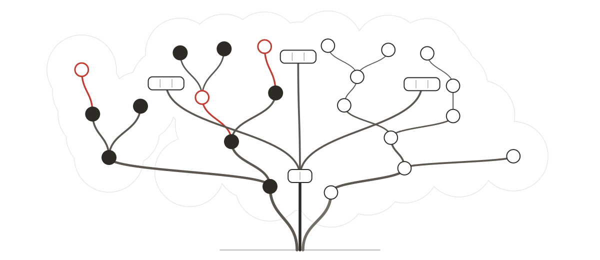
A red-black tree, a B-tree and a scapegoat tree all promise the same thing: finding or adding a key takes O(log n) time for n keys. On paper they are equivalent. That doesn’t help much if you have to choose one, so for an Algorithms group coursework at UCL we wrote implementations of all three in Python and benchmarked them, to understand the different advantages each one offers.
Left-leaning red-black tree
B-tree
Scapegoat tree
What we built
The notebook holds a left-leaning red-black tree, a B-tree and a scapegoat tree behind one shared interface, a generator for test data, and a framework that times every insert and every search. The B-tree takes a branching factor and the scapegoat tree takes an alpha, so we could sweep both. We used four kinds of input, each 10,000 five-character strings: random, sorted, “balanced” (median first) and “unbalanced”. Every run was repeated 1,000 times and averaged position by position, with outliers filtered out and a moving average drawn in Matplotlib.
What our results showed
On random strings the B-tree was the quickest to insert into and the slowest to search. The red-black tree was the reverse, and the scapegoat tree sat in the middle both times. Every time on these charts is a few microseconds, so the gaps are small.

In memory, smaller branching factors were faster to search: 35 and 50 were clearly slower than 5 and 20.

For the scapegoat tree, alphas of 0.5 and 0.6 were the slowest to insert with, and 0.7 to 0.9 ran close together. A higher alpha tolerates a deeper tree, so it rebuilds less often.

On the red-black tree, the four kinds of input gave almost the same insert times.

Each chart’s footnote says the moving average is plus or minus 200. The code smooths over 151 points, 75 either side, so read them that way.
What we concluded
On paper the three trees are equivalent. In our Python versions they weren’t, and no tree won outright. On random strings the B-tree suited insert-heavy work and the red-black tree suited lookups, with the scapegoat tree in between and an alpha to tune. Every operation took a few microseconds at 10,000 keys, so it was the constant factors, how much work each insert or search does, that decided the order, not the O(log n) they all share.
My takeaway
The theory behind an algorithm and its implementation often isn’t reflected in reality, because it can’t account for the deep complexity of a modern computer: scheduling, the memory hierarchy and how memory is managed. So it’s important to test several options on your real use case and make algorithm decisions empirically.